|
|
Volume 4 No.2, Spring 2001 |
ISSN# 1523-9926 |
|
|
Volume 4 No.2, Spring 2001 |
ISSN# 1523-9926 |
|
Using the TMS320C31 DSK
|
|||||||||||||||||||||||||||||||||||||||||||||||||||||||||||||||||||||||||||||||||||||||||||||||||||||||||
|
Wm. Hugh Blanton |
Mark
Rajai |
ABSTRACT
A course in microprocessors/microcontrollers is a common element of any electronic engineering technology program. Using the TMS320C31 DSP Starter Kit (DSK)1 in place of the typical microprocessor/microcontroller evaluation module (EVM) gives the instructor the ability to expand the course beyond the typical student experiences: instruction sets/assembly language, interrupts, I/O, etc. The DSK allows for these typical experiences while concurrently introducing the student to the topics associated with digital signal processing: sampling, aliasing, digital filters, digital control, Fast Fourier Transforms, convolution, etc. The student gets an introduction to one of the mainstays of electronic engineering technology (the microprocessor) and one of the fastest growing fields in electronics (digital signal processing) without adding additional courses to an often overly crowded curriculum.
INTRODUCTION
Like many State universities, East Tennessee State University is facing the dilemma of offering a sufficient number of technology courses within increasing structurally-mandated (state, institutional, and accrediting agencies) requirements. The effect of these mandated requirements is the decreasing proportion of technology courses offered in the undergraduate degree. This dilemma exacerbates the existing engineering technology curriculum conundrum of providing the breadth of coverage that affords the flexibility for professional growth while still furnishing the depth of coverage so that the graduate has the specific knowledge and skills to satisfy the immediate requirements of employers. To overcome these challenges, the successful electronic engineering technology curriculum must be creative in course offerings. At East Tennessee State University, we have moved from the traditional two-semester microprocessor/microcontroller sequence to a two-semester sequence in digital signal processing (DSP). This serves our program well as we move from a general electronic engineering technology program to a program that emphasizes digital communications. Using the Texas Instruments TMS320C31 DSP starter kit (DSK) that cost $99, we have the ability to teach many of the concepts associated with normal microprocessor technology while extending into one of the fastest growth areas in electronics.
The fundamentals of DSP theory (the application of sines and cosines) go back at least as far as the Babylonians.2 The modern history (Fourier series and transforms) of DSP began with Euler in 1748, and most of the famous mathematicians of the era (Bernoulli, Lagrange, Lacroix, Monge, and Laplace). Modern DSP use began expanding when Cooley somewhat serendipitously discovered the fast Fourier transform in the 1960s. As recently as a decade ago, DSP was more theory than practice. DSP was touted by a few experts, adopted by some early innovators, and reported in a few obscure articles. The only systems capable of doing signal processing were massive mainframes and supercomputers and even then, much of the processing was done off line rather than in real time. For example, seismic data was collected in the field, stored on magnetic tapes and then taken to a computing center, where a mainframe might take hours or days to digest the information.
DSP has gained greater acceptance in the electronics industry as more people understand its characteristics and applications. This greater acceptance has also resulted in a dramatic increase in the number of technical articles on the subject and an increase in its inclusion in college curricula. The first practical real-time DSP systems emerged in the late 1970s. Uses were limited to high-end technology, such as military and space systems. The economics began to change in the early 80s with the advent of single-chip DSP. With the emergence of application-specific, low-cost VLSI DSP chips, DSP applications have cropped up in areas such as telecommunications, control, automotive, military products, consumer products, multimedia applications, computer graphics and imaging, and data communications (Figure 1). A further advantage of using VLSI DSP chips is that the digital approach is not subject to environmental effects like component drift and aging.
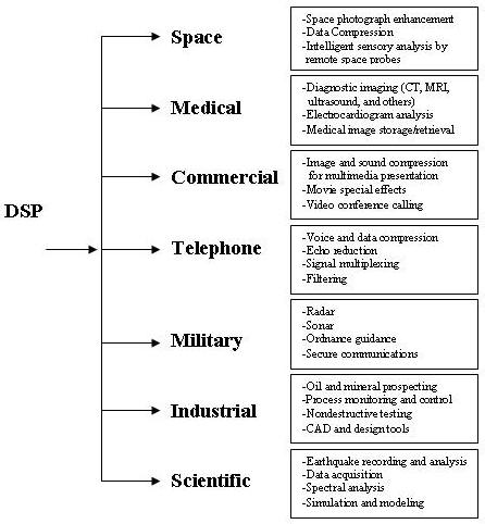
Figure 1. Application areas for DSP3
The downside to DSP continues to be the complicated mathematical methods needed to develop the particular DSP application. Although there are many good engineering technology programs and respect for engineering technology is growing in the industrial arena, there continues to be those who believe that the math capabilities of engineering technology students are limited. No one would oppose the reality that engineering programs are much more math intensive than engineering technology programs. These realities present a dilemma when introducing DSP into the technology curriculum. Because of the inherent mathematical rigor associated with DSP, some would argue that DSP is not a realistic topic for the engineering technology curriculum. The good news is that DSP design tools have been developed that reduce the mathematical harshness associated with DSP. Moreover, these tools are constantly becoming cheaper and easier to use. This combination of cheap, easy to use development tools has provided a critical mass of applications and sufficient formal language for discussion in mass engineering education, such as engineering technology programs.TWO-SEMESTER SEQUENCE
Whereas the microprocessor/microcontroller is a flexible general-purpose computer, the DSP processor is a dedicated computer that can race through a smaller range of functions at great speed. Nevertheless the first semester of the two-semester sequence in DSP is essentially the same as the first semester of the two-semester sequence in microprocessor technology. The student is introduced to the processor architecture including the address, data, and control buses along with the data, address and special purpose registers. The instruction set of the processor is examined in order to determine how data is manipulated and exchanged between memory and the processor. Memory management associated with interrupts and subroutines is discussed. The configuration of the system I/O along with their associated status registers is also examined.
Being a dedicated processor working at high speeds allows the opportunity to expand the traditional microprocessor-oriented concepts. For instance, the DSP processor works with a Harvard architecture as opposed to the Von Neuman architecture that is associated with many microprocessors. This allows for three operand instructions as well as parallel operations (specifically the multiply-accumulate (MAC) instruction that is the essence of DSP). As each new piece of signal data arrives, it must be multiplied, summed, and otherwise transformed according to complex formulas essentially using MAC instructions.
Because DSP is highly numerical and very repetitive, a number of mathematical topics must be addressed in the curriculum. In the first semester, the student reviews complex numbers and is introduced to Laplace and Z transforms. In order to alleviate some of the complexities of these mathematical issues, students are introduced to the mathematical programming package, MATLAB.
Like the standard second semester of a microprocessor sequence, the second semester of a DSP sequence involves applications, interfacing, and timing. Classical DSP applications work with real-world signals, such as sound and radio waves that originate in analog form. For instance, a DSP can filter the noise from a signal, remove unwanted interference, amplify certain frequencies and suppress others, encrypt information, or analyze a complex wave form into its spectral components. There are also DSP applications that do not require analog-to-digital conversion. The data is digital from the start and can be manipulated directly by the DSP. An example of this is computer graphics where DSP creates mathematical models of things such as images and scientific simulations.
DSP
We live in an analog world and perform analysis in a digital world. Thus a simple DSP processor contains an ADC to convert the signal from analog to digital, DSP processor to process the data, and a DAC converter to convert the signal back to analog (Figure 2).
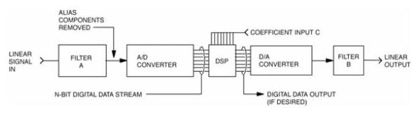
Figure 2. The DSP system
Because we sample the analog signal, an anti-aliasing filter normally precedes the ADC. Aliasing is a phenomenon related to sampling where higher frequencies are folded into lower frequencies (Figure 3). Thus, if a signal is sampled at rate of 40,000 samples/second, signals with frequencies greater than 20 KHz (half the sampling rate) will masquerade as lower frequencies. To prevent the folding of higher frequencies into lower frequencies, a low-pass filter (the anti-aliasing filter) eliminates the signals with frequencies greater than 20 KHz.
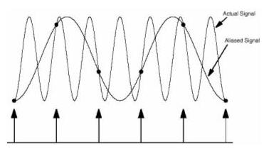
Figure 3. Aliasing
The DSP filter, usually a software algorithm, manipulates the data. The algorithm is normally based upon the Z-transform that is analogous to the Laplace transform used in the analysis of analog networks. The data is reconverted to analog using the DAC and the reconstruction filter at the output. The reconstruction filter is another low-pass filter used to smooth the output of the DAC output.
The TMS321C31 DSK (Figure 4) consists essentially of the DSP processor and analog interface chip (AIC). In addition there are two 1K ´ 32 RAMs, one 4K ´ 32 ROM, a 32-bit data bus, and a 24- bit address bus. Internally, the DSP processor has 8 general-purpose, extended-precision registers, 8 auxiliary registers, and 12 control registers, a DMA controller, one serial port, and two timers.
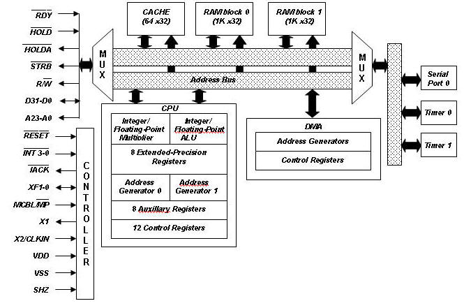
Figure 4. The Texas Instruments TMS320C31 functional diagram4
Analog input and output to the DSK is accomplished through the TLC32040 Analog Interface Chip5 (AIC). A block diagram is shown in Figure 5. Both the A/D and D/A convertors use 14 bits. The AIC allows you to sample two inputs ("IN" and "AUX IN"), at rates up to 19.2 kHz. The input signal may be filtered by a switched-capacitor bandpass filter for anti-aliasing. The input signal also has a user-selectable gain. The AIC also includes a low-pass switched-capacitor filter for output reconstruction. The use of switched-capacitor technology allows the frequency response of all of these filters to be set by the user.
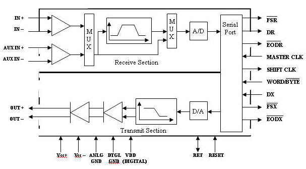
Figure 5. The TLC32040 AIC
Data transmission between the TMS320C31 and TLC 32040 occurs through two of the AIC’s serial port registers, the data receive (DR) and the data transmit (DX) registers (Figure 6). The AIC is controlled through the data transmit register. The two least significant bits (LSBs) are used for communication functions. When the two LSBs are zeros, normal transmission occurs, and when they are ones, secondary communication takes place. Secondary communication initializes and controls the AIC, allowing one secondary transmission before switching back.
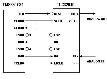
Figure 6. Interfacing between the TMS320C31 and TLC32040
The control word is 16 bits, and can have four different meanings depending on the least significant two bits, Table 1.
|
D15 |
D14 |
D13 |
D12 |
D11 |
D10 |
D9 |
D8 |
D7 |
D6 |
D5 |
D4 |
D3 |
D2 |
D1 |
D0 |
Mode |
|
x |
x |
TA Register |
x |
x |
RA Register |
0 |
0 |
0 |
||||||||
|
x |
TA' Register |
x |
RA' Register |
0 |
1 |
1 |
||||||||||
|
x |
TB Register |
x |
RB Register |
1 |
0 |
2 |
||||||||||
|
x |
x |
x |
x |
x |
x |
x |
x |
gain |
syn |
aux |
lb |
bp |
1 |
1 |
3 |
|
Table 1. TLC32040 Mode Control
The Mode bits are [D1 D0]. If the secondary transmission is done in Mode 0 [D1 D0] = [0 0], the 5 bits from D13-D9 are sent to the TA Register, and the 5 bits from D6-D2 are sent to the RA Register. Mode 1 [D1 D0] = [0 1] allows the programmer to fine tune registers TA and RA. If the transmission is done in Mode 2 [D1 D0] = [1 0], the TB Register is loaded from the 6 bits from D14 to D9, and the RB Register is loaded from bit D7-D2. If the transmission is done in Mode 3 [D1 D0] = [1 1], then the bits from D7-D2 have special meaning, as shown in Table 2.
| bit(s) | name | function |
| D2 | bp | =0
deletes bandpass filterz =1 inserts bandpass filter |
| D3 | lp | =0
disables loopback function =1 enables loopback function |
| D4 | aux | =0
disables AUX IN (uses IN) =1 enables AUX IN |
| D5 | syn | =0
asynchronous transmit/receive =1 synchronous transmit/receive |
|
[D7 D6] |
gain | =[0 0]
input gain=1 =[1 1] input gain=1 =[1 0] input gain=2 =[0 1] input gain=4 |
Table 2. Mode 3 [D1 D0] = [1 1] Bit Values
The D2 bit determines if the bandpass filter on the input is being used. Bit D3 enables a loopback function in which OUT+ and OUT- are internally connected to IN+ and IN- to test AIC functionality. Bit D4 specifies whether to use AUX IN or IN for the input to the AIC. Bit D5 is used to specify whether the receive and transmit section are synchronous. Bits D6 and D7 are used to specify the gain on the input. When the input gain is 4 ([D7 D6] = [0 1]), the maximum input (i.e., full scale for A/D convertor) is +1.5 volts. When the input gain is 2 ([D7 D6] = [1 0]), the maximum input is +3 volts. With an input gain of 1 ([D7 D6] = [0 0] or [1 1]), the maximum input voltage is +3 volts single ended and +6 differential. The reason for the difference is that the maximum voltage into the AIC is +3 volts, so if one of the inputs (IN -) is grounded (single ended input), the maximum input is +3 V. If neither input is grounded, one can be at +3 volts with the other one at -3 for a differential voltage of +6 V.
Most major DSP manufacturers (e.g., Motorola, Texas Instruments, Analog Devices, etc.) now provide low-cost ($100-$500) evaluation platforms for their DSP chips. Software almost always includes assemblers, linkers, and simulators. A C-compiler is often available. A major factor in choosing a DSP chip is whether it employs floating or fixed point math. Fixed-point chips are generally much cheaper, but floating point chips are easier to program (since one does not have to worry about certain effects the fixed-point math can produce).
A very popular program for DSP and engineering in general is MATLAB. One reason for MATLAB's popularity is the trend that MATLAB-based exercises and examples are being integrated into many engineering textbooks. The student version of the program may be purchased for about $100. Because there are a number of "toolboxes" including one for DSP, MATLAB can be used in several classes. Since MATLAB is a programming environment, a user can extend the functional capabilities of MATLAB by writing new modules called script files. Easy to use graphics are integrated into the software (Figure 7).
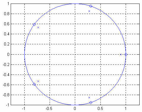
Figure 7. A MATLAB pole/zero plot
A LabView Digital Spectrum Analyzer (DSA) program, Figure 8, provides a cost-effective method of providing a spectrum analyzer for observing many of the labs used in DSP. For example, the DSA can be used to observe aliasing as a signal approaches the folding frequency. The DSA can also be used to observe the frequency spectrum of various signals and digital filters.
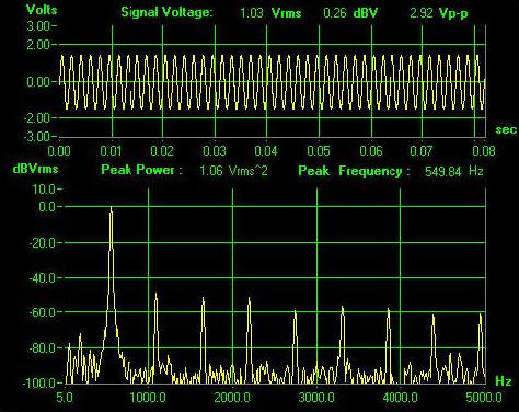
Figure 8. A LabView DSA
CONCLUSIONS
Once used primarily for academic research and futuristic military applications, digital signal processing has become a widely accessible commercial technology. In the last few years, a variety of high-performance, integrated DSPs have made digital signal processing technology easier and more affordable to use, particularly in low-end applications. DSPs are dedicated microprocessors. Because they are programmed and interfaced much like microprocessors, DSP theory provides a superb alternative for microprocessor theory, especially for programs that emphasize digital communications and digital control.
Also, software and development tools are more available so that students can easily become proficient in the use of DSP. Digital signal processing is not impossible to learn, it doesn't require an advanced degree in mathematics, and it really can be useful. There are now texts6,7 and other resources aimed at the non-engineer, and as a result it has never been easier to experiment with signal processing.
ACKNOWLEDGEMENTS
I would like to thank Texas Instruments and National Instruments for their ongoing support of the DSP lab at University. I also would like to thank for his support and wise counseling.
BIBLIOGRAPHY
[1] Chassaing, R., Digital Signal Processing: Laboratory Experiments Using C and the TMS320C31 DSK. NewYork: Wiley, (1999). [2] Oppeheim, A., Schafer, R., Buck, J., Discrete-Time Signal Processing. Upper Saddle River, NJ: Prentice-Hall (1999). [3] URL: http://www.dspguide.com [4] URL: http://www.ee.mtu.edu/faculty/schulz/new_page/Pages/EE422/lecture_notes [5] Texas Instruments, Analog Interface Circuits. Dallas, TX: Texas Instruments (1995). [6] Lyons, R., Understanding Digital Signal Processing. Upper Saddle River, NJ: Prentice-Hall (1996). [7] McClellan, J., Schafer, R., and Yoder, M., Dsp First: A Multimedia Approach. Upper Saddle River, NJ: Prentice-Hall(1998).