|
|
Volume 5 No.1, Winter 2003 |
ISSN# 1523-9926 |
|
|
Volume 5 No.1, Winter 2003 |
ISSN# 1523-9926 |
| Heidar A. Malki | Muhammad S. Anwar | |
| University of Houston | University of Houston | |
| 312 Technology Building | 312 Technology Building | |
| Houston, TX 77204-4022 | Houston, TX 77204-4022 | |
| malki@uh.edu | manwar32@hotmail.com |
Determination of lithofacies is prime factor in producing oil and gas for in oil and gas exploration. In this paper a neural network-based lithofacies determination technique is presented. This technique integrates both supervised and unsupervised neural networks. It presents a unique approach to well log analysis by acquiring target flags from unsupervised learning algorithm, and using those target flags for the training of back-propagation that belongs to a supervised neural network category. The back-propagation neural network is trained on two different sets of target flags. One set is obtained from a self-organizing map (unsupervised neural network model), and the other one is acquired from the well log analyst -- the human expert. The results of back-propagation neural network for both sets of target flags are then compared with each other. Targets obtained from self-organizing map neural network produce nearly 10% better results in identifying the lithofacies compared to well log analyst chosen target flags. The proposed method makes it easier to apply neural networks in well log analysis without prior knowledge of picking target flags.
The term log facies refers to the classes of rock that can be distinguishable according to the measurements of electromagnetic, acoustic, and nuclear properties. In other words, facies are the set of log responses that describe a bed by differentiating it from others [1]. Computer applications are used in the exploration of oil and gas fields both at the well site and in the office due to high speed processing of data. However, the applications for well log analysis, employing traditional computer programming, are not able to match the human ability to perceive trends, discrimination of groups, and anomalies within noisy data.
Pattern-recognition techniques are required to conclude the fundamental parameter values due to the variability in reservoir rock properties. The computational based application for well log analysis uses the statistical inference methods for calibration, prediction, and error analysis of reservoir properties. The statistical approaches have some limitations when dealing with non-linear and inseparable multiple regression [1].
The most frequently employed types of logging devices utilized in well bore are short spaced conductivity, natural gamma ray activity, bulk density, photoelectric effect, and neutron porosity. The selection of features to define log facies is a primary task in well bore analysis [3]. A geologist is able to classify facies from visual inspection of the log data curves, and his ability to recognize facies depends on experience and memory of the facies that exist, and their appearance in log curves in various positional surroundings.
Neural network technology provides a better solution for well log analysis due to its robustness over traditional estimation procedures of statistical regression. Neural networks trained for facies determination from well log do not replace the geologist, but assist the geologist in utilizing his/her time and experience more efficiently [2]. Recently, neural networks have been successfully applied to the determination of facies from well log data, and more work is in progress in order to find more effective utilization of this technology
The majority of previous works on well log analysis using neural network applications have been based on supervised training algorithms. In this work, a different approach to well log analysis, a self-organizing map (SOM) is used to pick target flags. The target flags are then used in the training of supervised back-propagation neural network to test the integrity of those flags. Target flags are found within the cluster nodes and refer to the data set that represents the facies.
In the experiments conducted in this work, target flags acquired from SOM are compared to well log analyst target flags in training back-propagation neural network. The effect of different parameters associated with SOM, such as resolution, the size of inhibition radius level, and the radii ratio of the size of inhibition/excitation are examined.
The self-organizing map is an unsupervised learning model that was introduced by Kohonen [4]. Most of the operating characteristics of the SOM resemble the biological functions of the brain. The architecture of the SOM consists of a collection of neurons located at nodes and connections among the nodes. Each node has an associated set of input weight. Since SOM is based on unsupervised learning (where desired target values are not provided to the network during the training phase).
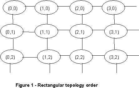
The SOM provides a topology-preserving mapping from high dimensional space to map units. The map unit is the output layer, a two-dimensional array of nodes that is fully connected to the input layer. The property of topology preservation refers to maintaining the relative distance between the points. The points that are closer to each other in input space are mapped close together on the map unit (output) in the SOM as shown in Figure 1. The distance between the map units can also be defined according to their topological relationship. Thus, SOM can be used as a cluster-analyzing tool of high dimensional data.
Another important property associated with SOM is its ability to generalize. This means that the network is able to recognize inputs that it has never encountered before. After training SOM, a vector is presented to the input layer, and the node whose weight vector is most similar to this input vector will be activated.
Some of the unique abilities of SOM are: 1) to perform visualization of data; 2) to provide informative representation of data; and 3) to compare whole data sets with each other. SOM has the capability of clustering the raw input data according to classification, so this property makes it a valuable tool for well log analysis. SOM will provide the cluster nodes to the log curves at each depth so that a geologist will be able to use these nodes for preliminary analyses. Neural networks have been successfully applied for well log analysis in recent years to name a few [5-14].
The software package, Thinking Log Module, used for training and testing purposes in this paper was selected from the Mind & Vision Computer Systems because of built-in features for analyzing well logs. This program acts as a simulator for both supervised and unsupervised neural network models. The SOM feature offers the user an “N-dimensional eyeball simulator” that is capable of seeing the data in N-dimensions without being biased.
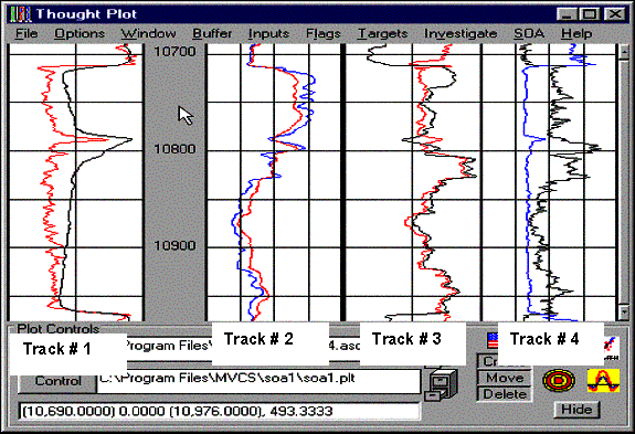
Well logs provide a recording of the variation of certain physical rock properties with depth. The data is acquired by lowering logging tools into the well. However, well logging data does not directly classify the rock properties. Well logging data assists in deducing the physical property of the rock by means of theoretical and empirical correlation. A suite of well log plots that consist of four tracks is shown in Figure 2.
· Track 1 contains spontaneous potential (SP) and Gamma ray (GRC) curves
· Track 2 represents resistivity logs (LOGSN and LOGILD)
· Track 3 contains neutron porosity curves (ROHB and NPHI)
· Track 4 holds calibration (CALI) and resistivity curve (LOGMLL) logs.
In this project, SOM is used to obtain cluster nodes from the well logging data, and then use those nodes as targets for the back-propagation neural network model. The eight input curves (SP, GRC, LOGSN, LOGILD, RHOB, NPHI, CALI, and LOGMLL), as shown in Figure 2, were selected for the training of SOM. The input data curves were normalized using the normalization feature of the program. Normalization of the input data may enhance the numerical accuracy [4].
Several trials of training SOM were conducted in order to determine the parameters for obtaining the optimal cluster nodes that represent all the facies in the data. After training, cluster nodes were picked from the output file generated by SOM. The parameters -- such as the number of input neurons, hidden and output neurons, the number of training cycles, and the bias level of the back-propagation -- were set to constant values.
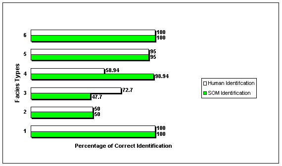
The back-propagation network was also trained using the target flags that were obtained from the well log analyst. The results of the back-propagation network for each facies type and the percent of correct identification during the testing phase when target flags were used from well log analysts are shown in Figure 6.
The optimal performance of the SOM is highly dependent on its parameters such as resolution, the size of inhibition radius level, and the radii ratio of inhibition/excitation. The preparation of the data for training requires manipulating these parameters in order to achieve satisfactory results because too little and/or too much change in the parameters could cause the network to converge inaccurately.
After several sets of experiments, it was observed that excitation signal level at 0.1, inhibition signal level at 0.03, resolution size of 18, and radii ratio of inhibition/excitation (Excitation = 1 and Inhibition = 2) contributed to achievement of the best target flags. Thus, the training of SOM was completed based on the above parameters, with the resulting target flags and seeds points (logs values at different depth) as shown in Table 1. This table also displays the corresponding values of density and neutron logs, and the number of facies classes associated according to depth.
An expert well log analyst gathered the classified interval values of the target curve and these values were used for comparison purposes through out this project. In Table 1, the target flags that were acquired from SOM training (at different depth values) represent all the corresponding facies from the data, plus unknown facies. This means that SOM is pointing to data that has not been classified by the well log analyst. Thus, SOM is not only able to extract the facies out of the well log data, but is also able to point toward data that might have some important value associated with it.
The architecture and other parameters associated with the back-propagation neural network were set before training the network. The network was composed of six (6) neurons for the input layer, 25 neurons for the hidden layer, and six (6) neurons for the output layer. These parameters were maintained during the training and testing phase of the back-propagation network for both sets of target flag values.
The back-propagation neural network was first trained and tested on the target flag values that were obtained from SOM. Next it was trained and tested on the target flag values that were provided by the well analyst. The cluster nodes or seeds acquired from SOM training were utilized as target flags for the back-propagation neural network in order to determine the effectiveness of SOM flag-picking ability in testing and training the supervised network. The back-propagation network was also trained and tested on the target flags that an expert human geologist picked from the same well log data. Table 2 represents the target flags and associated density and neutron log values that were picked by a well log analyst from the data.
Variation of parameters after several trials produced the best possible selection of values to be used for SOM training. SOM was trained using those parameter values, and produced the target flags that represented all the associated facies values of the data, as shown in Table 1.
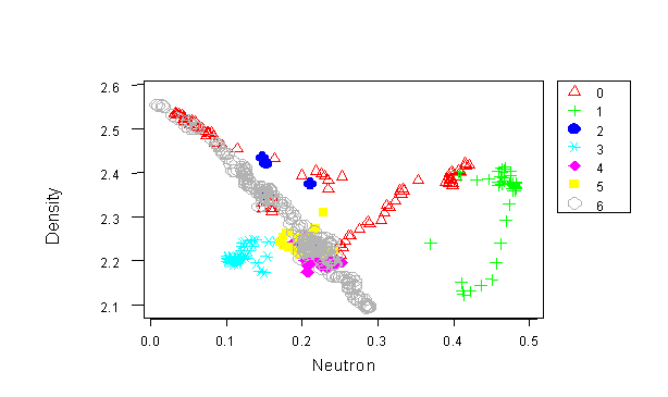
Figure 3 shows a scatter plot for density versus neutron log values for the entire well data. This figure indicated that facies (2, 3, 4, 5, and 6) types are in close proximity to one another. In other words, the data is highly correlated according to this scatter plot. Facies type 0, symbolized as a triangle on the plot, represents unclassified data that the well log analyst did not attempt to classify.
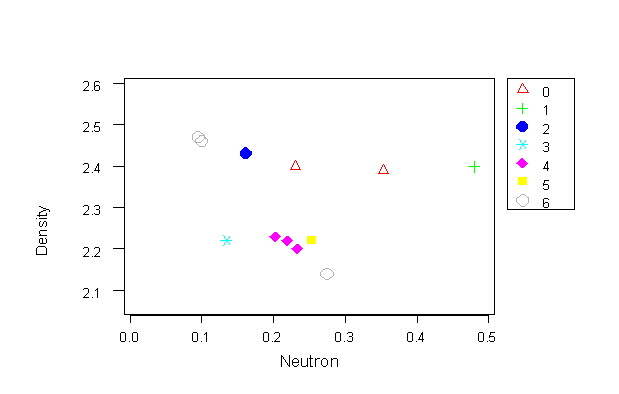
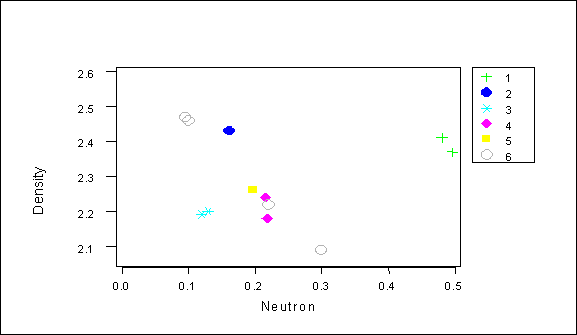
Figure 4 represents a scatter plot of density versus neutron log values for SOM-picked target flags. According to Figure 4, the SOM-picked target flags not only represent all the associated facies of data, but also point toward data that has not been classified by the well log analyst. This phenomenon indicates the cluster-analyzing capability of SOM. Figure 5 is a scatter plot of density versus neutron log values of target flags that have been chosen by the well log analyst after analyzing the well log suite data.
The comparison of the results of testing the back-propagation network with both sets of target flags is shown in Table 3. The back-propagation network correctly identified 85.88 % of the facies types during testing phase when SOM-picked target flag values were used. When human-picked target flag values were used, the network recognized 74.44 % of the facies types correctly by 74.44 % during the testing phase.
Figure 6 shows the comparison of the percentages of correct identification by the back-propagation network during the testing period of each facies types by SOM and human-selected target flag values. The network produced the same percentages of correctness for facies types 1, 2, 5, and 6 for both sets of target flag values as shown in Figure 6. The difference in the percentages of correct identification occurred for facies types 3 and 4. The network provided better percentages of correctness for facies type 4 when target flag values were used from SOM, and produced better results for correct identification of facies type 3 when human-picked target flag values were used. Overall the SOM-chosen target flag values yielded almost 10% percent better results for correct identification of the lithofacies types in the well log data compared to human-selected target flags.
In this project, it was observed that the performance of SOM depended on the selection of parameters such as: resolution, inhibition and excitation signal level, and inhibition/excitation radii ratio. However, it was difficult to assign an arbitrary constant value to those parameters because it depended upon the structure of the data. Several iterations of training the network were required in order to find those values for individual sets of data.
The performance of the back-propagation neural network was also dependent upon parameters such as learning rate, number of training cycles, and number of neurons in input layer. The determination of the best target seeds or flags from the well log data depended on the selection of parameters for SOM and normalization of well log curves.
The back-propagation neural network provided a higher percent correct yield rate (85.88%) for all the facies types when target flag values acquired from SOM were used, compared to a 74.44% correct yield rate when human-acquired target flag values were used. Thus, SOM-picked target flags produce nearly 10% better results in identifying the lithofacies for well log analysis compared to the well log analyst chosen target flags. Using the SOM in conjunction with the back-propagation network assist in developing fully automated stand-alone models for well log analysis
The result of this work reveals that by 1) selecting the best parameters associated with SOM and 2) normalizing the input log values, it is possible to achieve a better result from the back-propagation neural network. This does not mean that SOM will replace the geologist; rather SOM can be used by the geologist as an assisting tool for the interpretation of highly correlated data. This work also shows that the biological self-organizing paradigm in the retina can be expanded from two- dimensional to N-dimensional space in the computerized environment by using a neural network model.
|
Density |
Neutron |
Facies Type |
Target Flag Depth |
|
2.40 |
0.479 |
1 |
10698 |
|
2.43 |
0.161 |
2 |
10713 |
|
2.22 |
0.135 |
3 |
10731 |
|
2.22 |
0.220 |
4 |
10745.5 |
|
2.20 |
0.233 |
4 |
10755.5 |
|
2.23 |
0.203 |
4 |
10761 |
|
2.22 |
0.254 |
5 |
10793 |
|
2.40 |
0.231 |
Unknown |
10804.5 |
|
2.47 |
0.0945 |
6 |
10828 |
|
2.14 |
0.274 |
6 |
10879 |
|
2.46 |
0.099 |
6 |
10946 |
|
2.38 |
0.353 |
Unknown |
10969 |
|
Density |
Neutron |
Facies Type |
Target Flag Depth |
|
2.41 |
0.481 |
1 |
10695 |
|
2.37 |
0.496 |
1 |
10705 |
|
2.43 |
0.161 |
2 |
10713 |
|
2.19 |
0.120 |
3 |
10720 |
|
2.20 |
0.130 |
3 |
10730 |
|
2.24 |
0.216 |
4 |
10740 |
|
2.18 |
0.218 |
4 |
10770 |
|
2.26 |
0.197 |
5 |
10796 |
|
2.47 |
0.095 |
6 |
10828 |
|
2.22 |
0.220 |
6 |
10850 |
|
2.09 |
0.299 |
6 |
10875 |
|
2.46 |
0.099 |
6 |
10946 |
|
Facies |
Value of Occurrence |
SOM Identification |
Human Identification |
||
|
1 |
37 |
37 |
100 |
37 |
100 |
|
2 |
4 |
2 |
50 |
2 |
50 |
|
3 |
44 |
21 |
47.7 |
32 |
72.7 |
|
4 |
95 |
94 |
98.94 |
58 |
58.94 |
|
5 |
20 |
19 |
95 |
19 |
95 |
|
6 |
281 |
281 |
100 |
281 |
100 |
|
Total Average |
|
85.88 |
74.44 |
||
The authors would like to thank Mr. Jeff Baldwin from Mind & Vision Computer Systems for providing the software and providing expertise for this project. I would like to dedicate this paper to the memory of Muhammad S. Anwar who was killed in a car accident on the night of October 22, 2002 the same day when I contacted him to obtain his biography for this paper. May God rest his soul in peace. This work was supported in part from the Energy Lab at the University of Houston.
[1] John H. Doveton, “Geologic Log Analysis Using Computer Methods,” The American Association of Petroleum Geologists, 1994.
[2] Heidar Malki and Jeffrey Baldwin, “On the Comparison Results of the Neural Networks Trained Using Well-Logs from One service Company and Tested on Another Service Company’s Data,” pp. 1776-1779, IEEE International Conference on Neural Networks, Vol. III, 1993.
[3] Heidar Malki and Jeffrey Baldwin, “Determination of Lithofacies from Well-Logs Using Neural Networks," Journal of Engineering Technology, pp. 33-35, 1994.
[4] T. Kohonen, “Self-Organizing Maps,” Springer-Verlag Berlin Heidelberg, 1997.
[5] Jeffery Baldwin, “Using Simulated Bidirectional Associative Neural Network Memory with Incomplete Prototype Memories to Identify Facies from Intermittent Logging Data Acquired in Siliciclastic Depositional Sequence,” Paper presented at the 1991 Annual Technical Conference and Exhibition, October 6-9, 1991, Dallas, Texas.
[6] John Katsube, “Permeability Prediction with Computer Neural Network Modelling in the Venture Gas Field Offshore Eastern Canada,” http://agcwww.bio.ns/ca/hcmp/cnn/cnn.html.
[7] Quaglia Alfonso and Barbato Roberto, “Neural Network Applications to Upscale Core Data and Ancient Logs to Petrophysical Parameters of Flow Units, Caro Field, Eastern Venezuela,” SPWLA 39th Annual Logging Symposium, pp. 1-4, May 26-29, 1998.
[8] Terrilyn Olson, “Porosity and Permeability Prediction in Low-Permeability Gas Reservoirs From Well Logs Using Neural Networks,” pp. 563-572, Society of Petroleum Engineers, SPE 39964 85RGAW, April 1998.
[9] Juha Vesanto, “Data Mining Techniques Based on the Self-Organizing Map”, http://www.cis.hut.fi/projects/ide/publications/html/mastersJV97/index.html, May 26, 1997.
[10] E. A. Lovenzetti, “Predicting Lithology from Vp and Vs using Neural Networks.” Proceedings of the Society of Exploration Geologists Annual Meeting. October 24-27, 1992, New Orleans, La. 14-17.
[11] S. Mohaghegh, R. Arefi, and S. Ameri, “Petroleum Reservoir Characterization with the Aide of Artificial Neural Networks,” Journal of Petroleum Science and Engineering, Vol 16, pp. 263-274, 1996.
[12] P. M. Wong, D. J. Henderson, and L. J. Brooks, “Permeability Determination using Neural Networks in the Ravva Field, Offshore India,” SPE Reservoir Evaluation and Engineering Vol 1(2), pp. 99-104, 1998
[13] A. Al-Kaabi, and W. J. Lee, “Using Artificial Neural Nets to Identify the Well Test Interpretation Model, “ SPE Formation Evaluation, pp. 233-240, Sept. 1993,.
[14] R. Shelley, S. Stephenson, W. Haley, and E. Craig, “Red Fork Completion Analysis with the Aide of Artificial Neural Networks,” SPE 39963, Proceedings, Rocky Mountain Regional Meeting / Low Permeability Reservoir Symposium, April 5-8, Denver, CO, 1998.