|
|
Volume 4 No.1, Winter 2000 |
ISSN# 1523-9926 |
|
|
Volume 4 No.1, Winter 2000 |
ISSN# 1523-9926 |
|
Mikhail
M. Polonskii |
A procedure for complex systems simulation using MATLAB/SIMULINK
software is presented. As an example, an internal combustion engine was
chosen. The procedure is explained in detail to help for university students and
industry specialists in mastering this software. The models (MATLAB .m and
.mdl-files) developed are available for download.
The use of graphical dynamic system simulation software is becoming more popular as engineers strive to reduce the time to develop new control systems [ 1 ]. Dynamic system simulation software is an important tool for developing advanced reliable and high quality products and systems. Thus, the skill of complex systems simulation is the inherent goal of any engineer curriculum. In this article we show how to convert a set of differential non-linear time variant equations into easy to use MATLAB/SIMULINK graphical model. MATLAB/SIMULINK software has been chosen because many people use this software in both academia and industry. As the object of simulation we have selected an internal combustion engine.
The use of model based control methods designed to meet future emission and diagnostic regulations has also increased the need for validated engine models. A previously validated, nonlinear, mean torque predictive engine model is converted to MATLAB / SIMULINK to illustrate the benefits of a graphical simulation environment. The model is used to simulate a sequencial-fuel-injected, spark ignition engine and includes air and fuel dynamics in the intake manifold as well as the process delays inherent in a four stroke cycle engine. The engine model can be used in five ways [ 1]:
Although developed for a specific engine, the model is generic enough to
be used for a wide range of spark-ignition engines. Modular programming
techniques reduce model complexity by dividing the engine into
hierarchical subsystems. Further discussion supposes some basic knowledge of
MATLAB/SIMULINK of the reader.
The engine model for a four stroke spark ignition engine was developed by
Moskwa and Hendrick [ 2 ]. It was subsequently refined and used for different
studies. Here we use the model as it has been presented by Godbole [ 3, 4 ].
This is continuous time model with three state variables given by:
- the mass of air in intake manifold;
- the engine speed;
- mass flow rate of fuel entering combustion chamber.
The exhaust gas recirculation (ERG) system has not been included in this model.
The following state equation is obtained by applying law of conservation of mass
to the air flow in the intake manifold:
![]() ( 1 )
( 1 )
where
![]() =
mass of air in the intake manifold;
=
mass of air in the intake manifold;
![]() = mass rate of air in the intake manifold;
= mass rate of air in the intake manifold;
![]() =
mass rate of air entering the intake manifold;
=
mass rate of air entering the intake manifold;
![]() =
mass rate of air leaving the intake manifold and entering the combustion
chamber.
=
mass rate of air leaving the intake manifold and entering the combustion
chamber.
The mass of air entering the intake manifold is modeled as follows:
![]() ( 2 )
( 2 )
where
![]() =
the maximum flow rate corresponding to full open throttle,
=
the maximum flow rate corresponding to full open throttle,
![]() =
Normalized Throttle characteristic,
=
Normalized Throttle characteristic,
![]() =
Normalized Pressure Influence function.
=
Normalized Pressure Influence function.
Usually
![]() is
determined by an experiment and a data table is used in the simulation. Here we
use a curve fit as in [ 2 ]:
is
determined by an experiment and a data table is used in the simulation. Here we
use a curve fit as in [ 2 ]:
 ( 3 )
( 3 )
where
![]() =
the throttle angle.
=
the throttle angle.
The Normalized Pressure Influence function
![]() is
calculated as a function of manifold to atmosphere pressure ratio:
is
calculated as a function of manifold to atmosphere pressure ratio:
 ( 4 )
( 4 )
where
![]() =
intake manifold pressure,
=
intake manifold pressure,
![]() =
atmospheric pressure.
=
atmospheric pressure.
The intake manifold pressure
![]() and the mass of air
and the mass of air
![]() entering the intake manifold are modeled by ideal gas law:
entering the intake manifold are modeled by ideal gas law:
 ( 5 )
( 5 )
where
![]() =
constant value,
=
constant value,
![]() =
constant value,
=
constant value,
![]() =
constant value,
=
constant value,
![]() =
intake manifold volume
=
intake manifold volume
The flow of air from intake manifold to combustion chamber is given by
![]() ( 6 )
( 6 )
where
![]() =
engine angular velocity,
=
engine angular velocity,
![]() =
volumetric efficiency,
=
volumetric efficiency,
![]() is
given by
is
given by
 ( 7 )
( 7 )
The volumetric efficiency
![]() represents the effectiveness of engine's induction process. It is a complex
function of engine geometry and many engine parameters. It is normally modeled
by experimental data. Here the empirical formula given in [ 2 ]
represents the effectiveness of engine's induction process. It is a complex
function of engine geometry and many engine parameters. It is normally modeled
by experimental data. Here the empirical formula given in [ 2 ]
is used:
 ( 8 )
( 8 )
The dynamics of the fuel injection process is modeled as follows:
![]() ( 9 )
( 9 )
where
![]() =
fuel rate entering the combustion chamber,
=
fuel rate entering the combustion chamber,
![]() =
command fuel rate,
=
command fuel rate,
![]() =
effective fueling time
=
effective fueling time
constant, which is modeled as
 ( 10 )
where
![]() =
desired air/fiel ratio (tuning parameter),
=
desired air/fiel ratio (tuning parameter),
![]() =
constant value.
=
constant value.
The third state equation is obtained by applying Newton's second law to the
rotational dynamics of the engine:
![]() ( 11 )
( 11 )
where
![]() =
effective inertia of the engine,
=
effective inertia of the engine,
![]() =
engine indicated torque,
=
engine indicated torque,
![]() =
engine friction torque,
=
engine friction torque,
![]() =
accessories
=
accessories
torque.
In a four stroke engine, the process of torque production is discrete depending
on the engine speed. The model we used here is continuous, thus two delays were
introduced. The indicated torque is modeled by:
 ( 12 )
where,
![]() =
intake to torque production delay,
=
intake to torque production delay,
![]() =
spark to torque production delay,
=
spark to torque production delay,
![]() =
normalized air fuel
=
normalized air fuel
ratio influence function,
![]() =
normalized spark influence function,
=
normalized spark influence function,
![]() = the maximum torque production capacity of an engine for
= the maximum torque production capacity of an engine for
![]() =
1 and
=
1 and
![]() =
1. Here the following curve fit relation from [ 2 ] is used:
=
1. Here the following curve fit relation from [ 2 ] is used:
![]() ( 13 )
( 13 )
where
![]() =
actual air/fuel ratio of the mixture in the combustion chamber. With some
simplifying assumption, it will be given by:
=
actual air/fuel ratio of the mixture in the combustion chamber. With some
simplifying assumption, it will be given by:
 ( 14 )
Here the following curve fit relation from [ 2 ]is used:
![]() ( 15 )
( 15 )
where
![]() =
tuning parameter representing the spark advance from Top Dead Center (TDC),
=
tuning parameter representing the spark advance from Top Dead Center (TDC),
![]() =
the minimum spark advance from TDC for best torque. The engine friction torque
is curve fitted from experimental data [ 2 ] as
=
the minimum spark advance from TDC for best torque. The engine friction torque
is curve fitted from experimental data [ 2 ] as
![]() ( 16 )
( 16 )
Thus the engine model has tree states (
![]() ,
,
![]() ,
,
![]() ),
two control parameters (
),
two control parameters (
![]() ,
,
![]() )
and one control variable (
)
and one control variable (
![]() ). Table 1 summarizes the parameter values used for simulation, which had
been obtained for a 6-cilinders, 2.7 liter car engine.
). Table 1 summarizes the parameter values used for simulation, which had
been obtained for a 6-cilinders, 2.7 liter car engine.
|
|
0.1843 kg/s |
|
|
0.0038 m^3 |
|
|
0.0027 m^3 |
|
|
0.1454 kg m^2 |
|
|
498636 N m/ (kg/s) |
|
|
5.48/
|
|
|
1.3/
|
|
|
300 deg K |
|
|
28.84 g/mole |
|
|
8314.3 J/ mole deg K |
Table 1. Simulation Parameter Values
The complete model of the engine can be divided into air,
fuel and torque subsystems. This division is logical because the model is
based on the three state variables (
![]() ,
,
![]() ,
,
![]() ).
The air subsystem involves the equations from Equation 1 to Equation 8. The fuel
subsystem is determined by Equation 9 and Equation 10, and the torque
subsystem is defined by the
).
The air subsystem involves the equations from Equation 1 to Equation 8. The fuel
subsystem is determined by Equation 9 and Equation 10, and the torque
subsystem is defined by the
equations from Equation 11 to Equation 16.
To create the MATLAB/SIMULINK model of the engine, let us begin with the air
subsystem. The model should be hierarchical because this simplifies their use
and modification. Thus, we'll build the model through forming the subsystems
while the subsystems will be created by grouping simple blocks. First, we'll
transform Equations 6, 7 and 8 into MATLAB/SIMULINK model. Analyzing these
equations, it's easy to deduce that the inputs are (
![]() ,
,
![]() ,
,
![]() ,
,
![]() )
and the output is (
)
and the output is (
![]() ).
Three inputs for this subsystem are the model parameters (
).
Three inputs for this subsystem are the model parameters (
![]() ,
,
![]() ,
,
![]() )
and these parameters will be introduced as constants at the top level of
hierarchy of the model. Equations 6, 7 and 8 determine the air_3
subsystem of the air subsystem as shown in Figure 1.
)
and these parameters will be introduced as constants at the top level of
hierarchy of the model. Equations 6, 7 and 8 determine the air_3
subsystem of the air subsystem as shown in Figure 1.

Figure 1. The simulation diagram of the air_3 subsystem.
After creating this subsystem, we group all the blocks and entitle this
subsystem as air_3. The input and
output ports are labeled as the corresponding variables. The next step is to
convert Equation 5 into MATLAB/SIMULINK model. It is important to realize
that
![]() depends
on
depends
on
![]() ,
thus we'll get the air_2 subsystem as
follows:
,
thus we'll get the air_2 subsystem as
follows:

Figure 2. The simulation diagram of the air_2
subsystem.
The last part of the air subsystem model is air_1 and this involves Equations 2, 3 and 4. The MATLAB/SIMULINK corresponding model is present in Fig. 3.
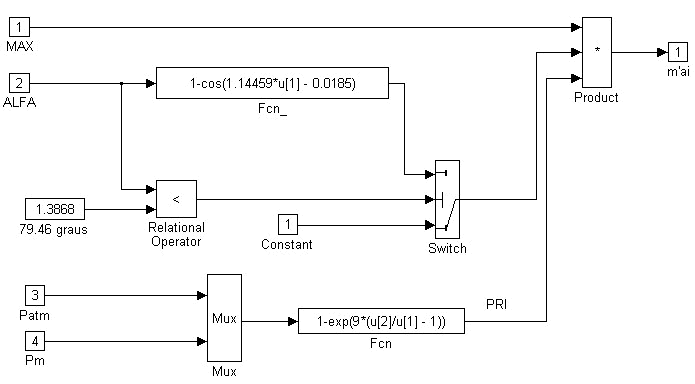
Figure 3. The air_1 subsystem's
MATLAB/SIMULINK model.
Now we can create the complete air subsystem model. This model joints the air_1, air_2, air_3 subsystems and involves one integrator and one sum block as appears in Fig. 4.
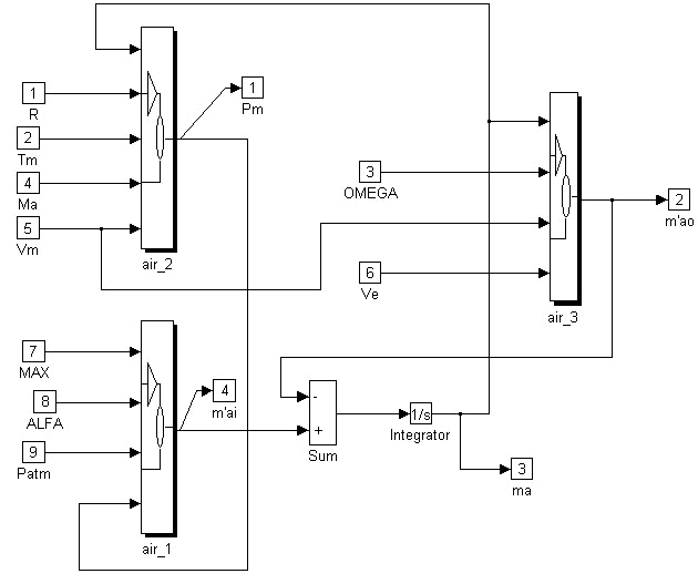
Figure 4. The complete air subsystem model.
Now we create the torque subsystem model. The model involves Equations
11, 12, 13, 14, 15 and 16. Obviously, this subsystem is complex and should be
divided into some subsystems. The first subsystem is torque_1.
This subsystem is based on the Equations 13, 14, 15 and calculates
![]() ,
,
![]() ,
,
![]() ,
,
![]() for Equation 12. Figure 5 shows this model.
for Equation 12. Figure 5 shows this model.
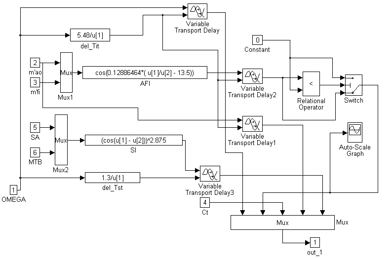
Figure 5. The torque_1 subsystem model.
This model involves four variable transport delay blocks according to
Equation 12. The point is to adjust the initial input value for each of these
blocks. The initial input for the Variable Transport Delay block (Figure 5) is
specified as 100 which is the initial engine velocity value. The initial input
for the Variable Transport Delay 1 block was adjusted to 0.014 because this
value had been obtained as the steady-state value for the velocity equals to 100
1/s. The initial input for the Variable Transport Delay 2 block was adjusted to
0.5 which is a reasonable value for cosine
function. The initial input for the Variable Transport Delay 3 block was
adjusted to 0.5 too. These initial specifications determine the
initial part of transient of the engine velocity.
The presence of the Constant, the Relational Operator and the Switch blocks
(Figure 5) should be commented. If we send the output of the Variable
Transport Delay 2 block directly to the corresponding input of the Mux block,
the transient of the engine velocity at the beginning of simulation
will tend to fall down. To discover the reason of such strange model dynamics we
can connect one Auto-Scale Graph ( for MATLAB v.4.2 ) to output of the
Variable Transport Delay 2 block. Then we can see that the output of the
Variable Transport Delay 2 block is oscillatory around the zero value. This
output is used as the factor for indicated torque calculation (Equation 12).
Thus, using the Constant, the Relational Operator and the Switch blocks
(Figure 5) we can clip the output of the Variable Transport Delay 2 block to
zero if this output becomes negative.
The torque_2 subsystem was created
to simulate Equations 11,12 and 16. Figure 6 shows the model.
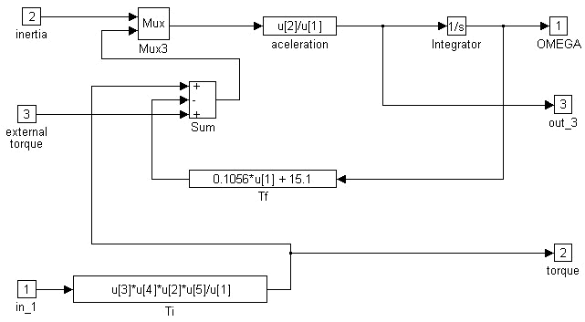
Figure 6. The torque_2 subsystem's model.
It is necessary to define the initial value of the Integrator (Figure
6) equal to 100, which is the initial value of the engine speed. If the initial
value of the Integrator is zero, the MATLAB zero-devision error is
generated.
The complete torque subsystem is shown in Figure 7
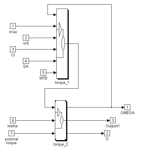
Figure 7. The torque subsystem model.
The last subsystem is the fuel subsystem and this involves Equations 9 and 10. First, we create the FUEL_1 subsystem model based on Equation 9 as shown in Figure 8.
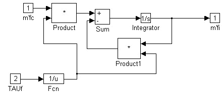
Figure 8. The MATLAB/SIMULINK FUEL_1 subsystem model.
This realization is better than one with numeric differentiation because of the absence of algebraic loop. The complete model of the fuel subsystem is done in Figure 9.
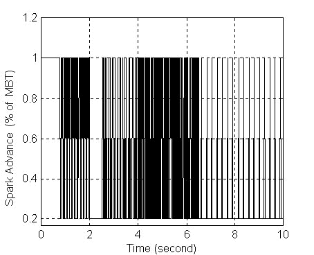
Figure 9. The model of the fuel subsystem.
Figure 10 shows the complete engine model with all the links between the subsystems.
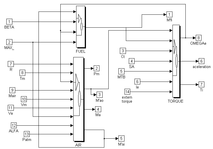
Figure 10. The whole model of the engine.
We can group these three subsystems into one and thus get the final version of the model. This version is shown in Figure 11.
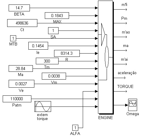
Figure 11. The final version of the engine MATLAB/SIMULINK model.
All of the simulation parameters are present at this upper level
of the model, which simplifies the model modification. The values of the
parameters
![]() ,
,
![]() and
and
![]() have been adjusted for the best engine torque production. Simulation of the
variations of these parameters can be useful to fuel injection and ignition
systems projects.
have been adjusted for the best engine torque production. Simulation of the
variations of these parameters can be useful to fuel injection and ignition
systems projects.
This model is available for download as eng.m
(for MATLAB v. 4.2) or as eng.mdl
(for MATLAB v.5).
Different types of simulation can be done using this MATLAB/SIMULINK engine
model. Here we simulate the open-loop dynamics of the engine. The first
simulation is executed for the engine when the external torque is zero,
the throttle angle is constant
![]() =
1 rad (Figure 11) and the engine velocity transient response is obtained. The
result is presented in Figure 12.
=
1 rad (Figure 11) and the engine velocity transient response is obtained. The
result is presented in Figure 12.
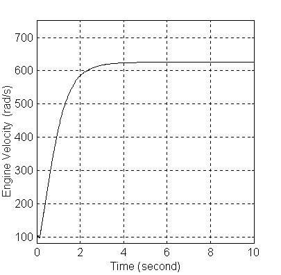
Figure 12. The engine velocity output (rad/s) in response to a unit throttle position input.
The velocity transient response shows some time delay at the beginning of the
process and the steady state velocity is about 620
rad/s. The initial time delay reflects the presence of the time
delay factors in Equation 12.
Another simulation is done for the throttle position
![]() =
0.6 rad when the external
torque = 10 sin t. The
engine velocity transient response is shown in Figure 13.
=
0.6 rad when the external
torque = 10 sin t. The
engine velocity transient response is shown in Figure 13.
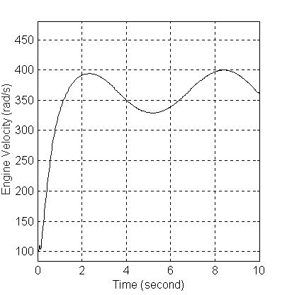
Figure 13. The engine
velocity output,
![]() =
0.6 rad, external torque
= 10 sin t.
=
0.6 rad, external torque
= 10 sin t.
This last simulation shows that the steady state velocity is about
370 rad/s and there are some velocity oscillations according to
the extern torque variations. Thus, to reduce the output sensitivity to extern
torque variations, it is necessary to implement some type of feedback control
scheme.
Now we'll see how the engine model can be used for closed-loop simulations. Let
us investigate the dynamics of a idle speed
relay controller. The model is shown in Figure 14.
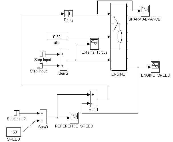
Figure 14. Idle engine speed control system
Here some of the engine parameters were hidden inside the
ENGINE subsystem. The controller controls spark advance angle, which is being
switched between 0.2 and 1, i.e. between 20% and 100% of the best torque spark
advance. During idle mode the engine works without load and their response is
very fast. This is the reason to control the spark advance, instead of the
throttle angle, because
![]() is more than 4 times greater than
is more than 4 times greater than
![]() (Table 1). The throttle angle
(Table 1). The throttle angle
![]() = 0.32 rad, it has been tuned by simulations and is contant. The REFERENCE
SPEED signal is shown in Figure 15.
= 0.32 rad, it has been tuned by simulations and is contant. The REFERENCE
SPEED signal is shown in Figure 15.
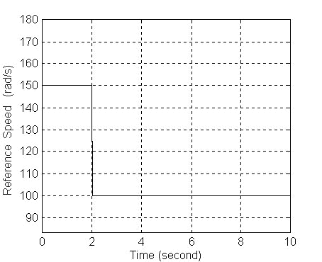
Figure 15. The REFERENCE SPEED signal.
Initially the REFERENCE SPEED is 150 rad/s and is greater
than the idle speed of the engine, which is 100 rad/s. If we try to simulate the
engine response, when the REFERENCE SPEED is 100 rad/s initially, the engine
stops due to engine friction torque and insufficient controller output.
The External Torque signal is shown in Figure 16. This signal has been chosen to
verify the system response under rapid external torque variations.
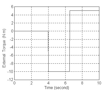
Figure 16. The External Torque signal.
The SPARK ADVANCE signal obtained by simulating the model (Figure 14) is shown in Figure 17.

Figure 17. The SPARK ADVANCE signal.
It can be seen that the frequency of the relay switching is
variable and depends on tne external torque value.
The ENGINE SPEED response is shown in Figure 18.
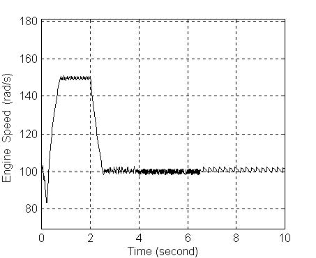
Figure 18. The ENGINE SPEED response.
We can see, that the engine response is quite fast and
precise. The system is not sensitive to external torque variations. The
procedure of the simulation has been as follows:
1. The open-loop dynamics of the engine has been simulated to
define the convenient constant
![]() value;
value;
2. The ralay controller has been added and switching limits
has been chosen;
3. Variable torque has beed added and final adjustment of the
ralay has been done.
The model ( Figure 14 ) is available for download as idle.m (for MATLAB v. 4.2).
CONCLUSIONS
This paper has presented the approach to complex systems
simulation using MATLAB/SIMULINK. As an example, the equations of the
four-stroke, 6-cilinder, 2.7 liter internal combustion engine has been chosen.
The "down-up" method of hierarchical model creation has been explained
step-by-step. Some simulations have been executed to demonstrate the open-loop
and closed-loop dynamics of the engine. The model can be used for closed-loop
cruise velocity control and injection/ignition systems simulations, too. It is
possible to integrate this model into the complete model of car dynamics [ 4 ].
The results presented here can be adopted to the electronics, mechatronics and
mechanics curricula to help in development of the skill of complex system
simulation.
[ 1 ] R.W. Weeks and J.J. Moskwa, "Automotive Engine Modeling for Real-time
Control Using MATLAB/SIMULINK", SAE paper No. 950417, 1995.
[ 2 ] J.J. Moskwa and J.K. Hedrick, "Modeling and validation of automotive engines for control algorithm development", ASME Journal of Mechanisms, Transmissions and Automation in Design, vol. 114, no. 2, pp. 278-285, 1992.
[ 3 ] D. Godbole and S. Karahan, "Automotive Powertrain Modeling, Simulation and Control using Integrated System's CASE Tools". Integrated Systems, Inc. Santa Clara, CA.
[ 4 ] D. Godbole, "Automotive Demos for Xmath. Automotive Suspension Design and Powertrain Speed Control". Intelligent Machines and Robotics Laboratory. University of California, Berkeley. godbole@robotics.eecs.berkeley.edu
_____________________________________________________________________________________________